3.4 Supply

[3.2 Demand] [3.3 Price Elasticity] [3.5 Production]

How do the actions of the Federal Reserve Bank influence the cost of obtaining loans for future investment projects? How do decisions of the Organization of Petroleum Exporting Countries (OPEC) affect energy costs? Will changes in national trade policy increase or decrease the prices of the agricultural commodities that a firm uses as inputs?

These questions all have at least one concept in common—supply. In competitive markets characterised by a large number of sellers that produce a similar product, the collective response to changes in the economic environment can have a significant impact on the prices of the goods they produce. The oil, banking and agricultural industries are examples of competitive markets for which analysis of supply is important and appropriate.

The supply of a good refers to the relation between the price of a good and the total quantity of the good that producers will be willing and able to offer at various prices, holding all other factors that affect producer decisions constant.

The law of supply states that other things being equal, as the price of a good increases, the quantity supplied of that good increases.

Check out the link here for an example of how the law of supply is observed.

The relation between price and quantity supplied holds because higher prices imply greater profit opportunities for producers, holding other things, such as input prices, constant. At higher prices, producers will usually devote greater resources to the production of that good.

Example: Supply of corn

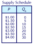
Assume an economic research service projects that farmers will supply 10 billion bushels of corn in the United States in the coming year, based on a price of $2 per bushel. Suppose that farmers would supply 5 billion bushels at a price of $1.50 per bushel and 15 billion bushels at a price of $2.50 per bushel.

By assuming the relation between price and quantity supplied continues in a similar fashion, you can illustrate this supply of corn on a graph. First, construct a supply schedule that lists various prices and the corresponding quantity (in billions of bushels) that farmers would supply at each price.

You can then simply plot the appropriate price-quantity pairs on the graph and connect them in a linear fashion to produce the supply line, or "market supply curve", as it is more generally known.

Read the following article to find out how changes in supply and demand affect prices of agricultural products, and how supply and demand for these products are interrelated.

You can express this relation between price and quantity supplied as a mathematical function. You can write the function in two equivalent ways. One way expresses price as a function of quantity supplied, as shown below.

The second way expresses quantity supplied as a function of price.

You read the function above as "quantity supplied is a function of price" not, "quantity supplied equals f times P". Quantity supplied "depends" on price; it is the dependent variable. P is the independent variable.

The following equation summarises the relation between price and quantity supplied represented by the Supply Schedule and Market Supply Curve:

Notice how this function reflects all of the information contained in the graph below. For example, inserting a quantity of 10 (billion) bushels for Q_s results in a price of $2, indicating that farmers would supply 10 (billion) bushels of corn at a price of $2 per bushel.

You can express the same relationship with quantity supplied on the left side of the function. Rearranging the same equation to isolate quantity supplied yields

Notice how the conversion maintains the underlying relation between price and quantity supplied. Substituting $2 for price results in Q_s = 10 (billion) as before.

is formally called a supply function, because it expresses quantity supplied as a function of price.

is called the inverse supply function to reflect the fact that it is the same supply relationship, just inverted. Because both equations represent the same supply relationship, economists commonly refer to either simply as the "supply function".

In practice, you will often work with the supply function expressed in terms of price because this is consistent with the way supply is treated graphically. That is, it reflects the placement of price on the y-axis and quantity supplied on the x-axis. The remainder of the course will adhere to this practice.

In general, the supply function for any linear supply relationship can be expressed as:

c = the y-intercept

d = slope of the function

Notice that c corresponds to the price at which quantity supplied becomes zero, and d measures the change in price that will generate a one-unit change in quantity supplied.

Other Factors That Influence Supply

The law of supply states that other things being equal, as the price of a good increases, the quantity supplied of that good increases. But what if one of the “other things” changes? For example, how would new legislation requiring more environmentally friendly (and more expensive) pesticides affect the supply of corn? And would a drop in the profitability of producing corn affect the supply of soybeans? Clearly, the supply relationship in each of these cases would change.

When an important factor other than the price of a good itself changes, a change in the supply of that good can occur. An increase in supply means producers are willing to supply more of a good at each price. Graphically, an increase in supply appears as a rightward (or upward) shift of the supply curve.

A decrease in supply means producers are not willing to sell as many units at each price as before. Graphically, a decrease in supply appears as a leftward shift of the supply curve.

Mathematically, a decrease or an increase in the y-intercept term c, indicates an increase or a decrease in supply, respectively:

Change in Quantity Supplied vs. Change in Supply

It is important to distinguish between a change in quantity supplied, which occurs when the price of the good alone changes, and a change in supply, which results from a change in one of the related factors other than price. When price changes, no "shift" in the underlying relationship occurs; you simply move to a higher or lower price-quantity pair along the same supply curve.

The primary factors that can cause a change in supply, or a shift in the supply curve, are:

· Input costs and taxes

· Technology and government regulations

· Profitability of substitutes in production

· Number of firms in the market

· Expectations

Click on the links below to find out more about each of these factors.

Input Costs and Taxes

Technology and Government Regulations

Profitability of Substitutes in Production

Number of Firms in the Market

Expectations

The animation below allows you to see how each of these factors affects the supply curve for the athletic shoe market.

Formally, the price elasticity of supply measures the percentage change in the quantity supplied (Q_s) of any good, X, relative to the percentage change in the price (P) of good X. Price elasticity of supply is written as

Measuring percentage change as the "change in" a variable divided by its original value, price elasticity of supply can be written mathematically as

For a linear supply curve (expressed in terms of price), such as P = c + dQ_s (where the parameter d is the slope), price elasticity of supply at a given point simplifies to

This is the point-slope formula for price elasticity of supply. You can use this formula to calculate the price elasticity at a given point on a linear supply curve.

Unlike price elasticity of demand, the price elasticity of supply is between zero and infinity because price and quantity supplied move in the same direction. Similar to the price elasticity of demand, the price elasticity of supply can be divided into the following three categories:

Example: Price Elasticity of Supply

Consider the linear supply function for pounds of tomatoes (expressed in terms of price)

P = the price per pound of tomatoes

Q_s = pounds (in thousands) of tomatoes supplied per day

What is the elasticity of supply at P = $4 per pound?

At P = $4, Q_s = 30 (thousand) pounds, so the price elasticity of supply is

Therefore, you could say that supply is elastic at a price of $4.

Elastic supply implies that producers respond to a price change with a relatively large increase or decrease in quantity supplied. The magnitude of the elasticity of supply depends mainly on the time frame under consideration and on the availability of resources necessary to produce the good. In particular, the shorter the time frame, the more inelastic supply tends to be, because producers have little time to change production decisions in response to a price change. For example, the supply of corn may be very inelastic over a period of several months but may be very elastic over a period of years. Also, if the production of a good requires a rare input or an unusual production process, supply will be more inelastic.

Topic Summary

In this topic, you have learnt how to

· explain the law of supply and why supply curves slope upwards

· express supply functions mathematically and graphically

· identify how changes in input costs and taxes, technology and government regulations, profitability of substitutes in production, number of firms in the market and expectations can cause changes in supply

· use price elasticity of supply to determine the sensitivity of quantity supplied to changes in price

Now go on to topic 3.5, “Production”.